40 how to show labels in excel chart
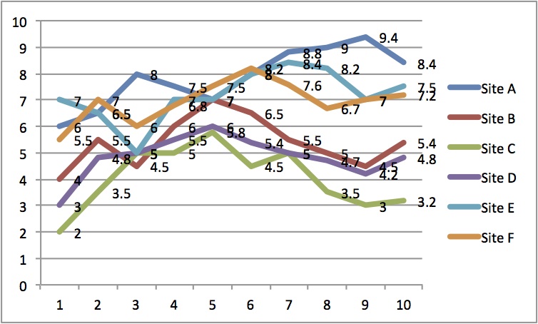
How to Show Percentage in Excel Pie Chart (3 Ways) Sep 08, 2022 · 2. Display Percentage in Pie Chart by Using Format Data Labels. Another way of showing percentages in a pie chart is to use the Format Data Labels option.We can open the Format Data Labels window in the following two ways.. 2.1 Using Chart Elements. To active the Format Data Labels window, follow the simple steps below.. Steps: peltiertech.com › broken-y-axis-inBroken Y Axis in an Excel Chart - Peltier Tech Nov 18, 2011 · For the many people who do want to create a split y-axis chart in Excel see this example. Jon – I know I won’t persuade you, but my reason for wanting a broken y-axis chart was to show 4 data series in a line chart which represented the weight of four people on a diet. One person was significantly heavier than the other three.
How to Add Labels to Scatterplot Points in Excel - Statology Step 3: Add Labels to Points. Next, click anywhere on the chart until a green plus (+) sign appears in the top right corner. Then click Data Labels, then click More Options…. In the Format Data Labels window that appears on the right of the screen, uncheck the box next to Y Value and check the box next to Value From Cells.

How to show labels in excel chart
Broken Y Axis in an Excel Chart - Peltier Tech Nov 18, 2011 · The primary axis then bisects the chart and the secondary is at the bottom of the chart. I usually hide the labels and often the tick marks for the primary axis. ... but my reason for wanting a broken y-axis chart was to show 4 data series in a line chart which represented the weight of four people on a diet. ... Broken Y Axis in an Excel Chart ... How to Show Percentage in Pie Chart in Excel? - GeeksforGeeks Jun 29, 2021 · It can be observed that the pie chart contains the value in the labels but our aim is to show the data labels in terms of percentage. Show percentage in a pie chart: The steps are as follows : Select the pie chart. Right-click on it. A pop-down menu will appear. Click on the Format Data Labels option. The Format Data Labels dialog box will appear. How To Add Data Labels In Excel - gr8idea.info Press f2 to move focus to the formula editing box; First add data labels to the chart (layout ribbon > data labels) define the new data label values in a bunch of cells, like this: Type the equal to sign; Click The Data Series You Want To Label. Next, highlight the cells in the range b2:c9. Click the chart to show the chart elements button.
How to show labels in excel chart. How to Insert Axis Labels In An Excel Chart | Excelchat We will go to Chart Design and select Add Chart Element Figure 6 - Insert axis labels in Excel In the drop-down menu, we will click on Axis Titles, and subsequently, select Primary vertical Figure 7 - Edit vertical axis labels in Excel Now, we can enter the name we want for the primary vertical axis label. Find, label and highlight a certain data point in Excel scatter graph Here's how: Click on the highlighted data point to select it. Click the Chart Elements button. Select the Data Labels box and choose where to position the label. By default, Excel shows one numeric value for the label, y value in our case. To display both x and y values, right-click the label, click Format Data Labels…, select the X Value and ... › easiest-waterfall-chart-in-excelWaterfall Chart in Excel - Easiest method to build. - XelPlus At this point it might look like you’ve ruined your Waterfall. Excel has added another line chart and is using that for the Up/Down bars. Don’t panic. Just right mouse click on any series and go to the Change Series Chart Type… From the Change Series Chart Type… options, find the Data Label Position Series and change it to a Scatter Plot. How to hide zero data labels in chart in Excel? - ExtendOffice If you want to hide zero data labels in chart, please do as follow: 1. Right click at one of the data labels, and select Format Data Labels from the context menu. See screenshot: 2. In the Format Data Labels dialog, Click Number in left pane, then select Custom from the Category list box, and type #"" into the Format Code text box, and click Add button to add it to Type list box.
How to Add Two Data Labels in Excel Chart (with Easy Steps) You can easily show two parameters in the data label. For instance, you can show the number of units as well as categories in the data label. To do so, Select the data labels. Then right-click your mouse to bring the menu. Format Data Labels side-bar will appear. You will see many options available there. Check Category Name. How to Use Cell Values for Excel Chart Labels - How-To Geek Mar 12, 2020 · The column chart will appear. We want to add data labels to show the change in value for each product compared to last month. Select the chart, choose the “Chart Elements” option, click the “Data Labels” arrow, and then “More Options.” Uncheck the “Value” box and check the “Value From Cells” box. Change axis labels in a chart - support.microsoft.com Right-click the category labels you want to change, and click Select Data. In the Horizontal (Category) Axis Labels box, click Edit. In the Axis label range box, enter the labels you want to use, separated by commas. For example, type Quarter 1,Quarter 2,Quarter 3,Quarter 4. Change the format of text and numbers in labels How To Add Data Labels In Excel - weekir.northminster.info To format data labels in excel, choose the set of data labels to format. Source: . Use a label for flexible placement of instructions, to emphasize text, and when merged cells or a specific cell location is not a practical solution. Click the chart to show the chart elements button. Source: superuser.com
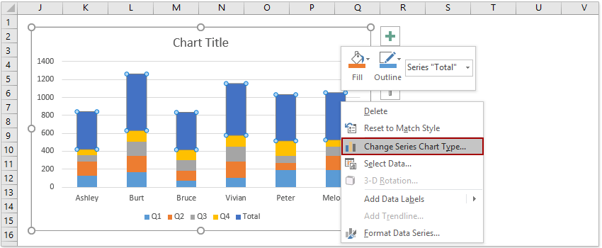
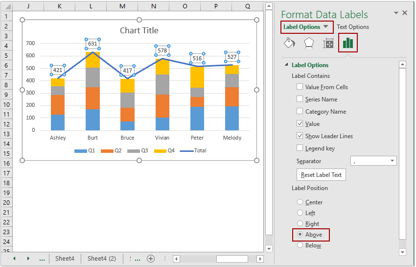
› excel › how-to-add-total-dataHow to Add Total Data Labels to the Excel Stacked Bar Chart Apr 03, 2013 · For stacked bar charts, Excel 2010 allows you to add data labels only to the individual components of the stacked bar chart. The basic chart function does not allow you to add a total data label that accounts for the sum of the individual components. Fortunately, creating these labels manually is a fairly simply process. How to add data labels in excel to graph or chart (Step-by-Step) Add data labels to a chart 1. Select a data series or a graph. After picking the series, click the data point you want to label. 2. Click Add Chart Element Chart Elements button > Data Labels in the upper right corner, close to the chart. 3. Click the arrow and select an option to modify the location. 4. How to show percentage in pie chart in Excel? - ExtendOffice Show percentage in pie chart in Excel. Please do as follows to create a pie chart and show percentage in the pie slices. 1. Select the data you will create a pie chart based on, click Insert > Insert Pie or Doughnut Chart > Pie. See screenshot: 2. Then a pie chart is created. Right click the pie chart and select Add Data Labels from the context ... How To Add Data Labels In Excel - happydanang.info After picking the series, click the data point you want to label. Click the chart to show the chart elements button. Required steps to print labels in excel. Source: . Required steps to print labels in excel. After that, select insert scatter (x, y) or bubble chart > scatter. Source:
Format Data Labels in Excel- Instructions - TeachUcomp, Inc.
How to Display Percentage in an Excel Graph (3 Methods) Then go to the More Options via the right arrow beside the Data Labels. Select Chart on the Format Data Labels dialog box. Uncheck the Value option. Check the Value From Cells option. Then you have to select cell ranges to extract percentage values. For this purpose, create a column called Percentage using the following formula: =E5/C5

Custom Excel Chart Label Positions • My Online Training Hub
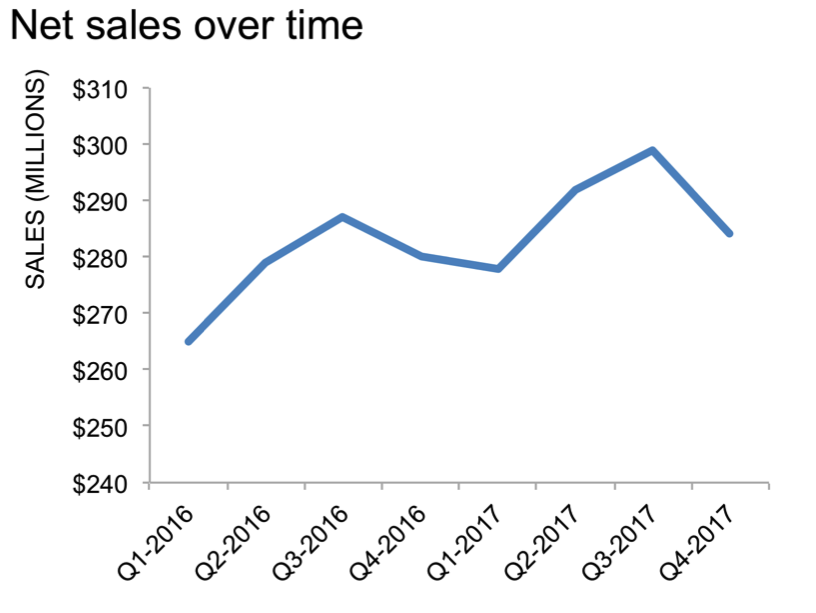
› examples › line-chartCreate a Line Chart in Excel (In Easy Steps) - Excel Easy Line charts are used to display trends over time. Use a line chart if you have text labels, dates or a few numeric labels on the horizontal axis. Use a scatter plot (XY chart) to show scientific XY data. To create a line chart, execute the following steps. 1. Select the range A1:D7.

Two-Level Axis Labels (Microsoft Excel)
Excel: How to Create a Bubble Chart with Labels - Statology Step 3: Add Labels. To add labels to the bubble chart, click anywhere on the chart and then click the green plus "+" sign in the top right corner. Then click the arrow next to Data Labels and then click More Options in the dropdown menu: In the panel that appears on the right side of the screen, check the box next to Value From Cells within ...

How to add live total labels to graphs and charts in Excel ...
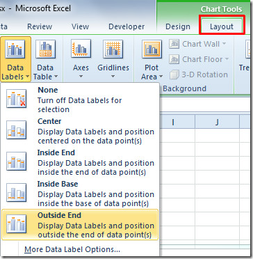
How to add or move data labels in Excel chart? - ExtendOffice In Excel 2013 or 2016. 1. Click the chart to show the Chart Elements button . 2. Then click the Chart Elements, and check Data Labels, then you can click the arrow to choose an option about the data labels in the sub menu. See screenshot: In Excel 2010 or 2007. 1. click on the chart to show the Layout tab in the Chart Tools group. See ...
Directly Labeling Excel Charts - PolicyViz
HOW TO CREATE A BAR CHART WITH LABELS INSIDE BARS IN EXCEL - simplexCT 7. In the chart, right-click the Series "# Footballers" Data Labels and then, on the short-cut menu, click Format Data Labels. 8. In the Format Data Labels pane, under Label Options selected, set the Label Position to Inside End. 9. Next, in the chart, select the Series 2 Data Labels and then set the Label Position to Inside Base.

microsoft excel - Adding data label only to the last value ...
How to add text labels on Excel scatter chart axis Add dummy series to the scatter plot and add data labels. 4. Select recently added labels and press Ctrl + 1 to edit them. Add custom data labels from the column "X axis labels". Use "Values from Cells" like in this other post and remove values related to the actual dummy series. Change the label position below data points.

Add or remove data labels in a chart
How To Add Data Labels In Excel - combo.northminster.info To get there, after adding your data labels, select the data label to format, and then click chart elements > data labels > more options. After picking the series, click the data point you want to label. Source: temotips.blogspot.com. Using excel chart element button to add axis labels. Click the chart to show the chart elements button.
How to add total labels to stacked column chart in Excel?
Change the format of data labels in a chart To get there, after adding your data labels, select the data label to format, and then click Chart Elements > Data Labels > More Options. To go to the appropriate area, click one of the four icons ( Fill & Line, Effects, Size & Properties ( Layout & Properties in Outlook or Word), or Label Options) shown here.
Excel 2010: Show Data Labels In Chart
How to Add Total Data Labels to the Excel Stacked Bar Chart Apr 03, 2013 · For stacked bar charts, Excel 2010 allows you to add data labels only to the individual components of the stacked bar chart. The basic chart function does not allow you to add a total data label that accounts for the sum of the individual components. Fortunately, creating these labels manually is a fairly simply process.

How to Add Data Labels to your Excel Chart in Excel 2013
How To Add Data Labels In Excel - ekinosan.info Click add chart element chart elements button > data labels in the upper. Next Open Format Data Labels By Pressing The More Options In The Data Labels. Make row labels in excel 2007 freeze for easier reading from . 47 rows add a label (form control) click developer, click insert, and then click label.
X-Axis labels in excel graph are showing sequence of numbers ...
How To Add Data Labels In Excel - newall.northminster.info After picking the series, click the data point you want to label. Click the chart to show the chart elements button. Required steps to print labels in excel. Source: . Required steps to print labels in excel. After that, select insert scatter (x, y) or bubble chart > scatter. Source:
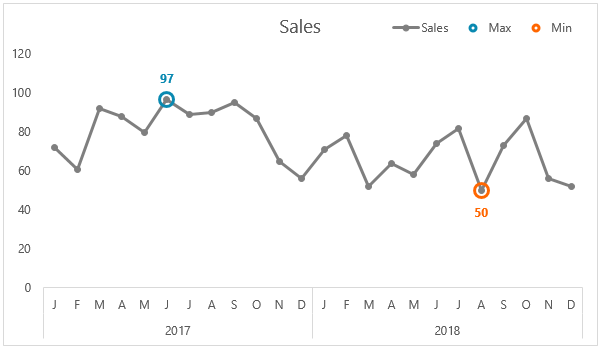
Label Excel Chart Min and Max • My Online Training Hub
How to Use Cell Values for Excel Chart Labels - How-To Geek Select the chart, choose the "Chart Elements" option, click the "Data Labels" arrow, and then "More Options." Uncheck the "Value" box and check the "Value From Cells" box. Select cells C2:C6 to use for the data label range and then click the "OK" button. The values from these cells are now used for the chart data labels.

Is there a way to add data labels as percentages on the ...
How to Make a PIE Chart in Excel (Easy Step-by-Step Guide) The best use of a Pie chart would be to show how one or two slices are doing as a part of the overall pie. For example, if you have a company with five divisions, you can use a Pie chart to show the revenue percent of each division. But if you have 20 divisions, it may not be the right choice. Instead, a column/bar chart would be better suited.

data visualization - How do you put values over a simple bar ...
trumpexcel.com › pie-chartHow to Make a PIE Chart in Excel (Easy Step-by-Step Guide) The best use of a Pie chart would be to show how one or two slices are doing as a part of the overall pie. For example, if you have a company with five divisions, you can use a Pie chart to show the revenue percent of each division. But if you have 20 divisions, it may not be the right choice. Instead, a column/bar chart would be better suited.

charts - Excel, giving data labels to only the top/bottom X ...
How to Add Axis Labels in Excel Charts - Step-by-Step (2022) - Spreadsheeto How to add axis titles 1. Left-click the Excel chart. 2. Click the plus button in the upper right corner of the chart. 3. Click Axis Titles to put a checkmark in the axis title checkbox. This will display axis titles. 4. Click the added axis title text box to write your axis label.

How to Add Axis Labels to a Chart in Excel | CustomGuide
Add or remove data labels in a chart - support.microsoft.com Click Label Options and under Label Contains, select the Values From Cells checkbox. When the Data Label Range dialog box appears, go back to the spreadsheet and select the range for which you want the cell values to display as data labels. When you do that, the selected range will appear in the Data Label Range dialog box. Then click OK.
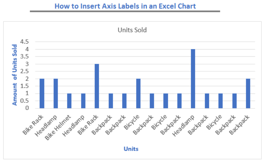
How to Insert Axis Labels In An Excel Chart | Excelchat
Data Labels in Excel Pivot Chart (Detailed Analysis) Next open Format Data Labels by pressing the More options in the Data Labels. Then on the side panel, click on the Value From Cells. Next, in the dialog box, Select D5:D11, and click OK. Right after clicking OK, you will notice that there are percentage signs showing on top of the columns. 4. Changing Appearance of Pivot Chart Labels

Add or remove data labels in a chart
How to Make a Pie Chart in Excel & Add Rich Data Labels to The Chart! Sep 08, 2022 · A pie chart is used to showcase parts of a whole or the proportions of a whole. There should be about five pieces in a pie chart if there are too many slices, then it’s best to use another type of chart or a pie of pie chart in order to showcase the data better. In this article, we are going to see a detailed description of how to make a pie chart in excel.

Excel charts: add title, customize chart axis, legend and ...
Waterfall Chart in Excel - Easiest method to build. - XelPlus At this point it might look like you’ve ruined your Waterfall. Excel has added another line chart and is using that for the Up/Down bars. Don’t panic. Just right mouse click on any series and go to the Change Series Chart Type… From the Change Series Chart Type… options, find the Data Label Position Series and change it to a Scatter Plot.

How to Use Cell Values for Excel Chart Labels
How to add axis label to chart in Excel? - ExtendOffice You can insert the horizontal axis label by clicking Primary Horizontal Axis Title under the Axis Title drop down, then click Title Below Axis, and a text box will appear at the bottom of the chart, then you can edit and input your title as following screenshots shown. 4.

How To Show Or Hide Data Labels On MS Excel? | My Windows Hub
Create a Line Chart in Excel (In Easy Steps) - Excel Easy Line charts are used to display trends over time. Use a line chart if you have text labels, dates or a few numeric labels on the horizontal axis. Use a scatter plot (XY chart) to show scientific XY data. To create a line chart, execute the following steps. 1. Select the range A1:D7.
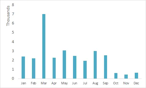
Show numbers in thousands in Excel as K in table or chart
› how-to-create-excel-pie-chartsHow to Make a Pie Chart in Excel & Add Rich Data Labels to ... Sep 08, 2022 · In this article, we are going to see a detailed description of how to make a pie chart in excel. One can easily create a pie chart and add rich data labels, to one’s pie chart in Excel. So, let’s see how to effectively use a pie chart and add rich data labels to your chart, in order to present data, using a simple tennis related example.

Solved: How to show all detailed data labels of pie chart ...
How to make a pie chart in Excel with words - profitclaims.com Select the range A1:D1, hold down CTRL and select the range A3:D3. 6. Create the pie chart (repeat steps 2-3). 7. Click the legend at the bottom and press Delete. 8. Select the pie chart. 9. Click the + button on the right side of the chart and click the check box next to Data Labels.

Add or remove data labels in a chart
Edit titles or data labels in a chart - support.microsoft.com On a chart, click the label that you want to link to a corresponding worksheet cell. On the worksheet, click in the formula bar, and then type an equal sign (=). Select the worksheet cell that contains the data or text that you want to display in your chart. You can also type the reference to the worksheet cell in the formula bar.

How to Add Data Labels to an Excel 2010 Chart - dummies
How To Add Data Labels In Excel - diffusori.info After picking the series, click the data point you want to label. Click the chart to show the chart elements button. Required steps to print labels in excel. Source: . Required steps to print labels in excel. After that, select insert scatter (x, y) or bubble chart > scatter. Source:

Bar charts with long category labels; Issue #428 November 27 ...
› excel-pie-chart-percentageHow to Show Percentage in Excel Pie Chart (3 Ways) Sep 08, 2022 · 2. Display Percentage in Pie Chart by Using Format Data Labels. Another way of showing percentages in a pie chart is to use the Format Data Labels option.We can open the Format Data Labels window in the following two ways.

424 How to add data label to line chart in Excel 2016
How to add data labels from different column in an Excel chart? Please do as follows: 1. Right click the data series in the chart, and select Add Data Labels > Add Data Labels from the context menu to add data labels. 2. Right click the data series, and select Format Data Labels from the context menu. 3.
Excel axis labels - supercategory — storytelling with data
How To Add Data Labels In Excel - gr8idea.info Press f2 to move focus to the formula editing box; First add data labels to the chart (layout ribbon > data labels) define the new data label values in a bunch of cells, like this: Type the equal to sign; Click The Data Series You Want To Label. Next, highlight the cells in the range b2:c9. Click the chart to show the chart elements button.
How to add total labels to stacked column chart in Excel?
How to Show Percentage in Pie Chart in Excel? - GeeksforGeeks Jun 29, 2021 · It can be observed that the pie chart contains the value in the labels but our aim is to show the data labels in terms of percentage. Show percentage in a pie chart: The steps are as follows : Select the pie chart. Right-click on it. A pop-down menu will appear. Click on the Format Data Labels option. The Format Data Labels dialog box will appear.

How to Add Total Data Labels to the Excel Stacked Bar Chart ...
Broken Y Axis in an Excel Chart - Peltier Tech Nov 18, 2011 · The primary axis then bisects the chart and the secondary is at the bottom of the chart. I usually hide the labels and often the tick marks for the primary axis. ... but my reason for wanting a broken y-axis chart was to show 4 data series in a line chart which represented the weight of four people on a diet. ... Broken Y Axis in an Excel Chart ...

Enable or Disable Excel Data Labels at the click of a button ...

Directly Labeling Your Line Graphs | Depict Data Studio
![Fixed:] Excel Chart Is Not Showing All Data Labels (2 Solutions)](https://www.exceldemy.com/wp-content/uploads/2022/09/Not-Showing-All-Data-Labels-Excel-Chart-Not-Showing-All-Data-Labels.png)
Fixed:] Excel Chart Is Not Showing All Data Labels (2 Solutions)

Adding rich data labels to charts in Excel 2013 | Microsoft ...

Improve your X Y Scatter Chart with custom data labels

How to Customize Your Excel Pivot Chart Data Labels - dummies
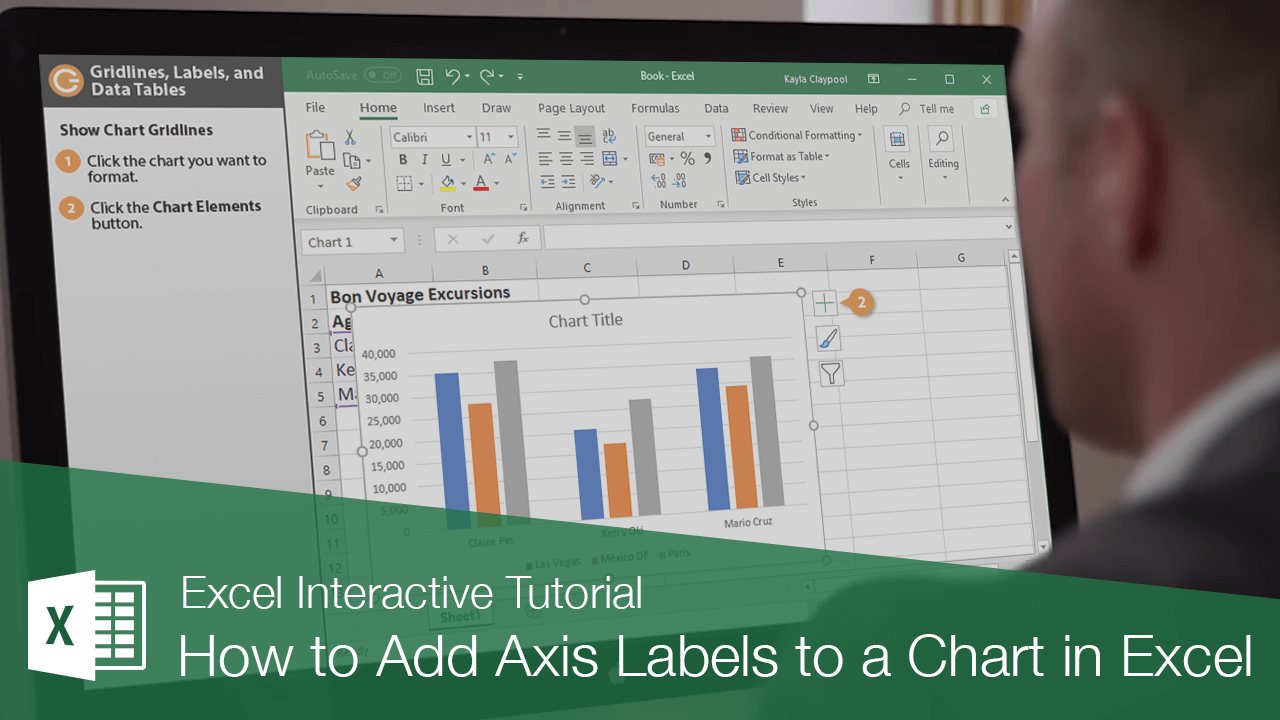
How to Add Axis Labels to a Chart in Excel | CustomGuide
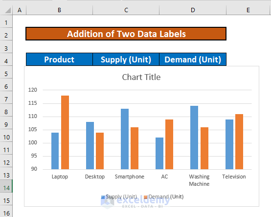
How to Add Two Data Labels in Excel Chart (with Easy Steps ...

Custom Data Labels with Colors and Symbols in Excel Charts ...
Directly Labeling Your Line Graphs | Depict Data Studio
Post a Comment for "40 how to show labels in excel chart"