42 how to add labels to excel chart
peltiertech.com › add-horizontal-line-to-excel-chartAdd a Horizontal Line to an Excel Chart - Peltier Tech Sep 11, 2018 · Let’s focus on a column chart (the line chart works identically), and use category labels of 1 through 5 instead of A through E. Excel doesn’t recognize these categories as numerical values, but we can think of them as labeling the categories with numbers. Adding Data Labels to Your Chart (Microsoft Excel) - ExcelTips (ribbon) Activate the chart by clicking on it, if necessary. Make sure the Design tab of the ribbon is displayed. (This will appear when the chart is selected.) Click the Add Chart Element drop-down list. Select the Data Labels tool. Excel displays a number of options that control where your data labels are positioned. Select the position that best fits ...
support.microsoft.com › en-us › officeAdd or remove data labels in a chart - support.microsoft.com Depending on what you want to highlight on a chart, you can add labels to one series, all the series (the whole chart), or one data point. Add data labels. You can add data labels to show the data point values from the Excel sheet in the chart. This step applies to Word for Mac only: On the View menu, click Print Layout.

How to add labels to excel chart
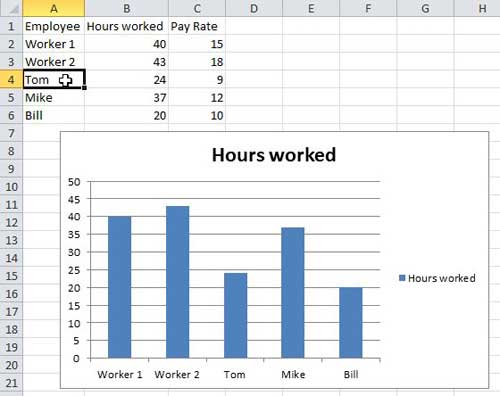
How to Use Cell Values for Excel Chart Labels - How-To Geek Select the chart, choose the "Chart Elements" option, click the "Data Labels" arrow, and then "More Options." Uncheck the "Value" box and check the "Value From Cells" box. Select cells C2:C6 to use for the data label range and then click the "OK" button. The values from these cells are now used for the chart data labels. HOW TO CREATE A BAR CHART WITH LABELS INSIDE BARS IN EXCEL - simplexCT 7. In the chart, right-click the Series "# Footballers" Data Labels and then, on the short-cut menu, click Format Data Labels. 8. In the Format Data Labels pane, under Label Options selected, set the Label Position to Inside End. 9. Next, in the chart, select the Series 2 Data Labels and then set the Label Position to Inside Base. Add data labels and callouts to charts in Excel 365 - EasyTweaks.com Step #1: After generating the chart in Excel, right-click anywhere within the chart and select Add labels . Note that you can also select the very handy option of Adding data Callouts.
How to add labels to excel chart. How to Add Data Labels to an Excel 2010 Chart - dummies Select where you want the data label to be placed. Data labels added to a chart with a placement of Outside End. On the Chart Tools Layout tab, click Data Labels→More Data Label Options. The Format Data Labels dialog box appears. Excel charts: add title, customize chart axis, legend and data labels Click anywhere within your Excel chart, then click the Chart Elements button and check the Axis Titles box. If you want to display the title only for one axis, either horizontal or vertical, click the arrow next to Axis Titles and clear one of the boxes: Click the axis title box on the chart, and type the text. How to Insert Axis Labels In An Excel Chart | Excelchat We will go to Chart Design and select Add Chart Element Figure 6 - Insert axis labels in Excel In the drop-down menu, we will click on Axis Titles, and subsequently, select Primary vertical Figure 7 - Edit vertical axis labels in Excel Now, we can enter the name we want for the primary vertical axis label. chandoo.org › wp › change-data-labels-in-chartsHow to Change Excel Chart Data Labels to Custom Values? May 05, 2010 · We all know that Chart Data Labels help us highlight important data points. When you “add data labels” to a chart series, excel can show either “category” , “series” or “data point values” as data labels. But what if you want to have a data label that is altogether different, like this:
› documents › excelHow to add data labels from different column in an Excel chart? This method will introduce a solution to add all data labels from a different column in an Excel chart at the same time. Please do as follows: 1. Right click the data series in the chart, and select Add Data Labels > Add Data Labels from the context menu to add data labels. 2. Link a chart title, label, or text box to a worksheet cell On a chart, click the title, label, or text box that you want to link to a worksheet cell, or do the following to select it from a list of chart elements. Click a chart. This displays the Chart Tools tabs. Note: The names of the tabs within Chart Tools differs depending on the version of Excel you are using. spreadsheeto.com › axis-labelsHow to Add Axis Labels in Excel Charts - Step-by-Step (2022) How to Add Axis Labels in Excel Charts – Step-by-Step (2022) An axis label briefly explains the meaning of the chart axis. It’s basically a title for the axis. Like most things in Excel, it’s super easy to add axis labels, when you know how. So, let me show you 💡. If you want to tag along, download my sample data workbook here. Add / Move Data Labels in Charts - Excel & Google Sheets Adding Data Labels Click on the graph Select + Sign in the top right of the graph Check Data Labels Change Position of Data Labels Click on the arrow next to Data Labels to change the position of where the labels are in relation to the bar chart Final Graph with Data Labels
How To Create Labels In Excel - canada-eh.info Click inside the chart area to display the chart tools. Address Envelopes From Lists In Excel. It may be in a folder called microsoft. Go to mailing tab > select. Creating labels from a list in excel, mail merge, labels from excel. After Inserting A Chart In Excel 2010 And Earlier Versions We Need To Do The Followings To Add Data Labels To The ... How to Add Axis Labels to a Chart in Excel | CustomGuide Add Data Labels. Use data labels to label the values of individual chart elements. Select the chart. Click the Chart Elements button. Click the Data Labels check box. In the Chart Elements menu, click the Data Labels list arrow to change the position of the data labels. › excel › how-to-add-total-dataHow to Add Total Data Labels to the Excel Stacked Bar Chart Apr 03, 2013 · For stacked bar charts, Excel 2010 allows you to add data labels only to the individual components of the stacked bar chart. The basic chart function does not allow you to add a total data label that accounts for the sum of the individual components. Fortunately, creating these labels manually is a fairly simply process. Custom Chart Data Labels In Excel With Formulas - How To Excel At Excel Follow the steps below to create the custom data labels. Select the chart label you want to change. In the formula-bar hit = (equals), select the cell reference containing your chart label's data. In this case, the first label is in cell E2. Finally, repeat for all your chart laebls.
Custom Excel Chart Label Positions • My Online Training Hub
How to Add X and Y Axis Labels in Excel (2 Easy Methods) Then go to Add Chart Element and press on the Axis Titles. Moreover, select Primary Horizontal to label the horizontal axis. In short: Select graph > Chart Design > Add Chart Element > Axis Titles > Primary Horizontal. Afterward, if you have followed all steps properly, then the Axis Title option will come under the horizontal line.

Add data labels to your Excel bubble charts | TechRepublic
How to add arrows to line / column chart in Excel Add arrows to column chart in excel. Step 1. In the first, we must create a sample data for chart in an excel sheet in columnar format as shown in the below screenshot. Step 2. Then, select the cells in the A1:B10 range. Click on Insert tool bar and select bar chart>2-D column to display the graph for the above sample data.

microsoft excel - How to add comment column as special labels ...
How to add text labels on Excel scatter chart axis 3. Add dummy series to the scatter plot and add data labels. 4. Select recently added labels and press Ctrl + 1 to edit them. Add custom data labels from the column "X axis labels". Use "Values from Cells" like in this other post and remove values related to the actual dummy series. Change the label position below data points.
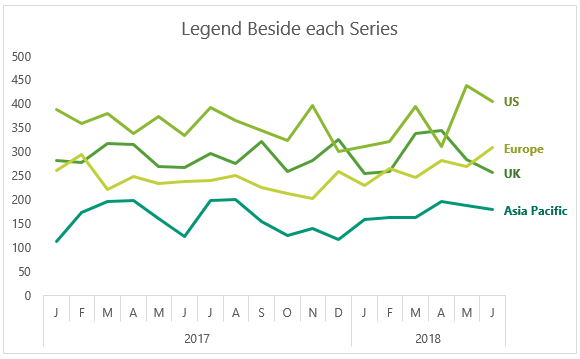
Dynamically Label Excel Chart Series Lines • My Online ...
How to Add Labels to Scatterplot Points in Excel - Statology Step 3: Add Labels to Points. Next, click anywhere on the chart until a green plus (+) sign appears in the top right corner. Then click Data Labels, then click More Options…. In the Format Data Labels window that appears on the right of the screen, uncheck the box next to Y Value and check the box next to Value From Cells.

How to add or move data labels in Excel chart?
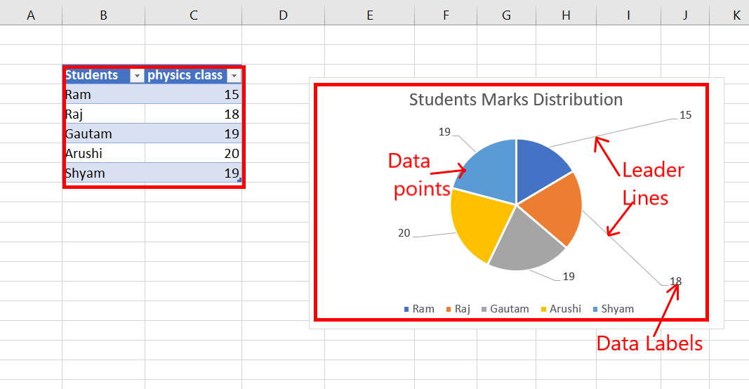
› how-to-create-excel-pie-chartsHow to Make a Pie Chart in Excel & Add Rich Data Labels to ... Sep 08, 2022 · In this article, we are going to see a detailed description of how to make a pie chart in excel. One can easily create a pie chart and add rich data labels, to one’s pie chart in Excel. So, let’s see how to effectively use a pie chart and add rich data labels to your chart, in order to present data, using a simple tennis related example.

How-to Use Data Labels from a Range in an Excel Chart - Excel ...
How to add data labels in excel to graph or chart (Step-by-Step) Add data labels to a chart 1. Select a data series or a graph. After picking the series, click the data point you want to label. 2. Click Add Chart Element Chart Elements button > Data Labels in the upper right corner, close to the chart. 3. Click the arrow and select an option to modify the location. 4.

How to Place Labels Directly Through Your Line Graph in ...
Add a DATA LABEL to ONE POINT on a chart in Excel Click on the chart line to add the data point to. All the data points will be highlighted. Click again on the single point that you want to add a data label to. Right-click and select ' Add data label ' This is the key step! Right-click again on the data point itself (not the label) and select ' Format data label '.

Change the format of data labels in a chart
Data Labels in Excel Pivot Chart (Detailed Analysis) Before adding the Data Labels, we need to create the Pivot Chart in the beginning. We can create a Pivot Chart from the Insert tab. To do this, go to Insert tab > Tables group. Then in the dialog box, select the range of cells of the primary dataset., here the range of cells is B4:J23. And select the New Worksheet in the next option.

Add Data Labels for Total to Stacked Columns in #Excel | wmfexcel
how to add data labels into Excel graphs - storytelling with data You can download the corresponding Excel file to follow along with these steps: Right-click on a point and choose Add Data Label. You can choose any point to add a label—I'm strategically choosing the endpoint because that's where a label would best align with my design. Excel defaults to labeling the numeric value, as shown below.
How to Change Horizontal Axis Labels in Excel 2010 - Solve ...
How to Add Data Labels in Excel - Excelchat | Excelchat After inserting a chart in Excel 2010 and earlier versions we need to do the followings to add data labels to the chart; Click inside the chart area to display the Chart Tools. Figure 2. Chart Tools Click on Layout tab of the Chart Tools. In Labels group, click on Data Labels and select the position to add labels to the chart. Figure 3.

264. How can I make an Excel chart refer to column or row ...
How to add label to axis in excel chart on mac - WPS Office How to add label to axis in excel online, 2016 and 2019 1. After choosing your chart, go to the Chart Design tab that appears. Axis Titles will appear when you choose them with the drop-down arrow next to Add Chart Element. Choose Primary Horizontal, Primary Vertical, or both from the pop-out menu. 2.

Add a Data Callout Label to Charts in Excel 2013 – Software ...
Excel: How to Create a Bubble Chart with Labels - Statology To add labels to the bubble chart, click anywhere on the chart and then click the green plus "+" sign in the top right corner. Then click the arrow next to Data Labels and then click More Options in the dropdown menu: In the panel that appears on the right side of the screen, check the box next to Value From Cells within the Label Options ...

Apply Custom Data Labels to Charted Points - Peltier Tech
How do you add total data labels in Excel? How to Add Total Data Labels to the Excel Stacked Bar Chart. Step 1: Create a sum of your stacked components and add it as an additional data series (this will distort your graph initially) Step 2: Right click the new data series and select "Change series Chart Type…". Step 3: Choose one of the simple line charts as your new Chart Type.
How to add axis labels in Excel - Quora
How to add axis label to chart in Excel? - ExtendOffice Select the chart that you want to add axis label. 2. Navigate to Chart Tools Layout tab, and then click Axis Titles, see screenshot: 3.

Add label to Excel chart line • AuditExcel.co.za MS Excel ...
How to add or move data labels in Excel chart? - ExtendOffice 1. Click the chart to show the Chart Elements button . 2. Then click the Chart Elements, and check Data Labels, then you can click the arrow to choose an option about the data labels in the sub menu. See screenshot:
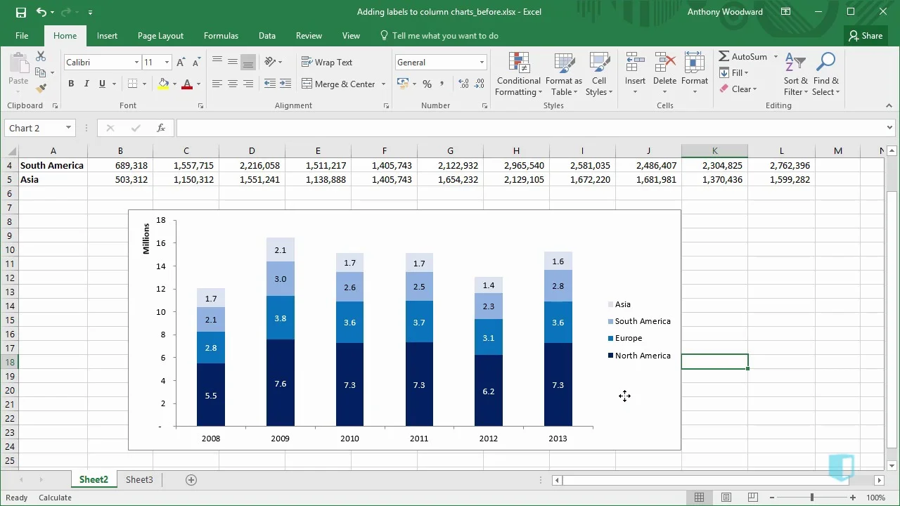
Adding Labels to Column Charts | Online Excel - KPMG Tax - Digital Now Course Training
Add data labels and callouts to charts in Excel 365 - EasyTweaks.com Step #1: After generating the chart in Excel, right-click anywhere within the chart and select Add labels . Note that you can also select the very handy option of Adding data Callouts.

How to Insert Axis Labels In An Excel Chart | Excelchat
HOW TO CREATE A BAR CHART WITH LABELS INSIDE BARS IN EXCEL - simplexCT 7. In the chart, right-click the Series "# Footballers" Data Labels and then, on the short-cut menu, click Format Data Labels. 8. In the Format Data Labels pane, under Label Options selected, set the Label Position to Inside End. 9. Next, in the chart, select the Series 2 Data Labels and then set the Label Position to Inside Base.

Add or remove data labels in a chart
How to Use Cell Values for Excel Chart Labels - How-To Geek Select the chart, choose the "Chart Elements" option, click the "Data Labels" arrow, and then "More Options." Uncheck the "Value" box and check the "Value From Cells" box. Select cells C2:C6 to use for the data label range and then click the "OK" button. The values from these cells are now used for the chart data labels.
How do i add Data labels on the Pareto Line for the Pareto ...
Text Labels on a Horizontal Bar Chart in Excel - Peltier Tech

Add Custom Labels to x-y Scatter plot in Excel - DataScience ...

Change the format of data labels in a chart

Add or remove data labels in a chart

424 How to add data label to line chart in Excel 2016

Adding rich data labels to charts in Excel 2013 | Microsoft ...

Two-Level Axis Labels (Microsoft Excel)

How to add or move data labels in Excel chart?

Chart axes, legend, data labels, trendline in Excel - Tech Funda
How to Add Leader Lines in Excel? - GeeksforGeeks

Adding rich data labels to charts in Excel 2013 | Microsoft ...

Excel: How to Create a Bubble Chart with Labels - Statology
/simplexct/BlogPic-idc97.png)
How to Create a Bar Chart With Labels Inside Bars in Excel

Custom data labels in a chart

Add or remove data labels in a chart

Directly Labeling Excel Charts - PolicyViz

Add or remove data labels in a chart

Custom Data Labels with Colors and Symbols in Excel Charts ...

microsoft excel - Adding data label only to the last value ...

Adding rich data labels to charts in Excel 2013 | Microsoft ...

How To Show Or Hide Data Labels On MS Excel? | My Windows Hub

How to Add and Remove Chart Elements in Excel
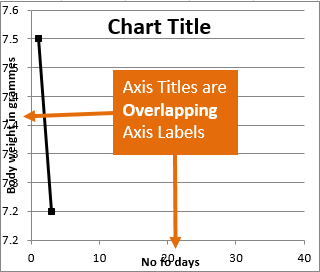
Resize the Plot Area in Excel Chart - Titles and Labels Overlap
Post a Comment for "42 how to add labels to excel chart"