44 accept labels in formulas excel 2013
Illustrated Course Guide: Microsoft Excel 2013 Intermediate Lynn Wermers · 2013 · ComputersQUiCK Tip Because a table acts much like a database, database functions allow you to summarize table data in a variety of ways. When working with a sales ... How to Create a Barcode in Excel | Smartsheet Use the barcode font in the Barcode row and enter the following formula: ="*"&A2&"*" in the first blank row of that column. Then, fill the formula in the remaining cells in the Barcode row. The numbers/letters you place in the Text row will appear as barcodes in the Barcode row. See step-by-step instructions for Excel 2013 here.
Enhanced Microsoft Excel 2013: Illustrated Complete Elizabeth Reding, Lynn Wermers · 2015 · ComputersUse the Find & Select feature to replace the Accounting label in cell A5 with ... Create a formula in cell E4 that calculates the value of the items in ...

Accept labels in formulas excel 2013
superuser.com › questions › 815798microsoft excel - Have Pivot Chart show only some columns in ... It doesn't look like this topic has been addressed recently on forums, but a workaround I found was to format the unwanted series in the pivot chart to 1) have 100% overlap, 2) no fill, and 3) no outline. That resulted in the appearance of removing the unwanted series while still maintaining the data link. I'm using excel 2013. Excel- Labels, Values, and Formulas - WebJunction Simple Formula: Click the cell in which you want the answer (result of the formula) to appear. Press Enter once you have typed the formula. All formulas start with an = sign. Refer to the cell address instead of the value in the cell e.g. =A2+C2 instead of 45+57. That way, if a value changes in a cell, the answer to the formula changes with it. Excel Table: Header with formula - Microsoft Community Click in your table, select Design under Table Tools on the ribbon, and then uncheck "Header Row". That should allow you to enter a formula in the cell above your table data. This method can be used when you are willing to sacrifice the "Sort" ability of Header Row after you protect the sheet.
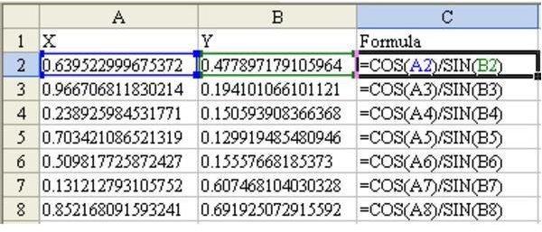
Accept labels in formulas excel 2013. The Do's and Don'ts of Entering Data in Excel - Lifewire Format numbers in the heading cells as text or create text labels by preceding each number with an apostrophe ( ' ) such as '2012 and '2013. The apostrophe doesn't show in the cell, but it changes the number to text data. Keep Units in the Headings Don't enter currency, temperature, distance, or other units into each cell with the number data. Excel 2013 CONCATENATE function won't display result In that case, simply changing the cell format to General afterwards does not change the type of the cell contents. You must also "re-enter" the formula. You can accomplish that simply by selecting the cell, pressing F2, then Enter. In the future, be sure cells are not formatted as Text before entering a formula. Excel 2013: Label deconfliction in labeled scatter plot This formula then goes into G2 to create the series with labels below the point, which is all remaining values: =IF(ISERROR(F2),E2,NA()) One trick is just required to make the autofilter work on the data. Because we used the SUBTOTAL formula, Excel thinks the last row is a subtotal row and automatically excludes it from the autofilter, even if ... Adding rich data labels to charts in Excel 2013 - Microsoft 365 Blog To add a data label in a shape, select the data point of interest, then right-click it to pull up the context menu. Click Add Data Label, then click Add Data Callout . The result is that your data label will appear in a graphical callout. In this case, the category Thr for the particular data label is automatically added to the callout too.
Names in formulas - support.microsoft.com Select the cell, range of cells, or nonadjacent selections that you want to name. Click the Name box at the left end of the formula bar. Name box Type the name you want to use to refer to your selection. Names can be up to 255 characters in length. Press ENTER. Note: You cannot name a cell while you are changing the contents of the cell. Repeat All Item Labels In An Excel Pivot Table - MyExcelOnline You can then select to Repeat All Item Labels which will fill in any gaps and allow you to take the data of the Pivot Table to a new location for further analysis. STEP 1: Click in the Pivot Table and choose PivotTable Tools > Options (Excel 2010) or Design (Excel 2013 & 2016) > Report Layouts > Show in Outline/Tabular Form Excel 2013 Formulas - Page 335 - Google Books Result John Walkenbach · 2013 · ComputersAn essential requirement of the IRR function is that there must be both negative and ... it also affects the labels in row 5, which contain formulas that ... Formula Bar | How To Excel Enter data into any cell. Select the cell where you want to enter your data and start typing. As you type the data notice the data also appear in the Formula Bar. To accept the data either click the Check Mark or press Enter. To discard the data either click the X or press Esc. The process for entering a formula is the same except all formulas ...
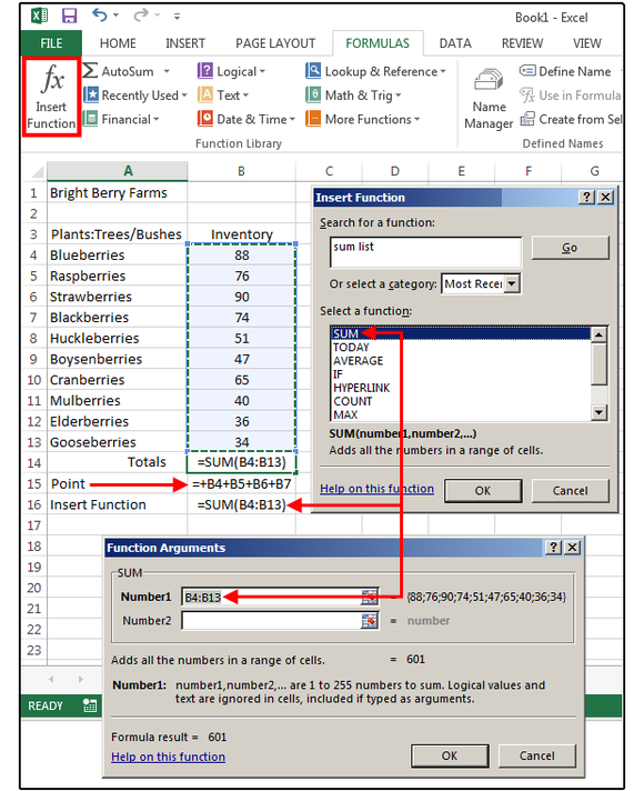
How to Display a Label Within a Formula on Excel - YouTube How to Use the AutoSum Feature in Microsoft Excel 2013 Excel will select a range of adjacent cells for you. If Excel choose the wrong range of cells, just use your mouse to click and drag over the correct range of cells to use in the formula. 2. Click the "AutoSum" button again or press the "Enter" key on your keyboard to accept the formula. 3. How to Print Labels From Excel - EDUCBA Navigate towards the folder where the excel file is stored in the Select Data Source pop-up window. Select the file in which the labels are stored and click Open. A new pop up box named Confirm Data Source will appear. Click on OK to let the system know that you want to use the data source. Again a pop-up window named Select Table will appear. How to Format the X and Y Axis Values on Charts in Excel 2013 To change the alignment and orientation of the labels on the selected axis, click the Size & Properties button under Axis Options on the Format Axis task pane. Then, indicate the new orientation by clicking the desired vertical alignment in the Vertical Alignment drop-down list box and desired text direction in the Text Direction drop-down list.
Excel Tips and Tricks: 2012
Use defined names to automatically update a chart range - Office Microsoft Excel 97 through Excel 2003. On the Insert menu, click Chart to start the Chart Wizard. Click a chart type, and then click Next. Click the Series tab. In the Series list, click Sales. In the Category (X) axis labels box, replace the cell reference with the defined name Date. For example, the formula might be similar to the following ...
How to Use Excel Like a Pro: 18 Easy Excel Tips, Tricks, & Shortcuts
How to use AutoFill in Excel - all fill handle options - Ablebits In Excel 2010-2013 click File -> Options -> Advanced -> scroll to the General section to find the Edit Custom Lists… button. Since you already selected the range with your list, you will see its address in the Import list from cells: field. Press the Import button to see your series in the Custom Lists window.
Discover How To Assign A Formula To A Name With This Excel Tutorial
Excel 2016 - How to Use Formulas and Functions To do this, we are going to click Insert Function on the Ribbon under the Formulas tab. Once again, we enter "average of cells" in the "Search for a Function field," then click the Go button. Select Average, then click OK. Excel prompts us for our arguments. The arguments are the cells or values that we want to use to calculate the function.

One of the keys to all happiness, is to have a bad memory...: Excel
How to Use Templates and Outlines in Excel 2013 In the Choose Commands From dropdown menu, choose View Menu, as circled in red below. Click on Custom Views to select it. Next, click the Add button. Click OK. You will then see a Custom Views icon displayed in the Quick Access Toolbar. We have highlighted it below. Click the downward arrow beside the icon.
Your Excel formulas cheat sheet: 22 tips for calculations and common tasks | PCWorld
Define and use names in formulas - support.microsoft.com Select Formulas > Create from Selection. In the Create Names from Selection dialog box, designate the location that contains the labels by selecting the Top row,Left column, Bottom row, or Right column check box. Select OK. Excel names the cells based on the labels in the range you designated. Use names in formulas
Excel 2003 Printing Options
How to mail merge and print labels from Excel - Ablebits You are now ready to print mailing labels from your Excel spreadsheet. Simply click Print… on the pane (or Finish & Merge > Print documents on the Mailings tab). And then, indicate whether to print all of your mailing labels, the current record or specified ones. Step 8. Save labels for later use (optional)
/labels_1-56a8f70f3df78cf772a242a0.gif)
Using Labels to Simplify Your Excel 2003 Formulas
How to add data labels from different column in an Excel chart? In the Format Data Labels pane, under Label Options tab, check the Value From Cells option, select the specified column in the popping out dialog, and click the OK button. Now the cell values are added before original data labels in bulk. 4. Go ahead to untick the Y Value option (under the Label Options tab) in the Format Data Labels pane.
Advanced Excel Formulas - DCOUNT Function Description With Example
How to Display a Formula Result in a Text Box in Excel 2010 Step 3: Enter the formula whose result you want to display in the text box. Step 4: Click the Insert tab at the top of the window. Step 5: Click the Text Box button in the Text section of the navigational ribbon. Step 6: Draw your text box where you want it to display in the worksheet. Step 7: Click inside the text box once to select it, then ...

Where Do I Put The Label? In Excel – Excel-Bytes
excel - Change format of all data labels of a single series at once ... Click anywhere in formula bar above. Don't change anything. Click the 'tick icon' just to the left of the formula bar. Go straight back to the same data series and right mouse click, and choose add data labels This has worked in Excel 2016. Purely by luck I worked this out saving a great deal of time and frustration. Share Improve this answer
Post a Comment for "44 accept labels in formulas excel 2013"