38 how to show data labels as percentage in excel
How to show percentage in Excel - Ablebits Jan 13, 2015 · To apply the percent format to a given cell or several cells, select them all, and then click the Percent Style button in the Number group on the Home tab: Even a faster way is pressing the Ctrl + Shift + % shortcut (Excel will remind you of it every time you hover over the Percent Style button). Data label in the graph not showing percentage option. only ... Data label in the graph not showing percentage option. only value coming Team, Normally when you put a data label onto a graph, it gives you the option to insert values as numbers or percentages. In the current graph, which I am developing, the percentage option not showing. Enclosed is the screenshot.
Make a Percentage Graph in Excel or Google Sheets Change Labels to Percentage. Click on each individual data label and link it to the percentage in the table that was made. Final Percentage Graph in Excel. The final graph shows how each of the items change percentage by quarter. Make a Percentage Graph in Google Sheets. Copy the same data on Google Sheets . Creating a Graph. Highlight table ...
How to show data labels as percentage in excel
how to calculate turnover percentage in excel - hojosoun.com Invoice template excel with vat. Gross Profit Percentage = ((Total Sale - Cost of Goods Sold) / Total sales) * 100 Gross Profit Percentage = (($3,000,000 - $650,000) / $3,000,000) * 100 Gross Profit Percentage = 78.33% In the Format Data Labels task pane, untick Value and tick the Percentage option to show only percentages. Change the format of data labels in a chart - Microsoft Support To get there, after adding your data labels, select the data label to format, and then click Chart Elements > Data Labels > More Options. To go to the appropriate area, click one of the four icons ( Fill & Line, Effects, Size & Properties ( Layout & Properties in Outlook or Word), or Label Options) shown here. How to visualize percentage progress in Excel Open the options for the Data Bar formatting you added and check Show Bar Only option. Click the OK buttons to apply the setting. Colored Icons Conditional Formatting has icons as well to visualize percentage progress. The first set of icons we want to show are color-based icons.
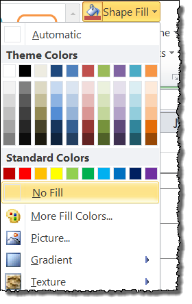
How to show data labels as percentage in excel. How to show values in data labels of Excel Pareto Chart ... 2) Move Value data series to 2nd Axis 3) Change Value data series Fill from Automatic to No Fill 4) Change 2nd Vertical Axis Labels to None 5) Add Data Labels to Value data series Hope this helps. Steve=True D dendres New Member Joined Aug 1, 2015 Messages 14 Aug 3, 2015 #3 Hi Steve=True, Thank you for the help. How to Change Excel Chart Data Labels to Custom Values? First add data labels to the chart (Layout Ribbon > Data Labels) Define the new data label values in a bunch of cells, like this: Now, click on any data label. This will select "all" data labels. Now click once again. At this point excel will select only one data label. Go to Formula bar, press = and point to the cell where the data label ... How to show data label in "percentage" instead of - Microsoft ... Jul 05, 2012 · Select Format Data Labels Select Number in the left column Select Percentage in the popup options In the Format code field set the number of decimal places required and click Add. (Or if the table data in in percentage format then you can select Link to source.) Click OK Regards, OssieMac Report abuse 8 people found this reply helpful · Percent charts in Excel: creation instruction Now we show the percentage of taxes in the diagram. Click the right mouse button. In the dialog box select a task "Add Data Labels". The values from the second column of the table will be on the parts of the circle: Once again right click on the chart and select the item "Format Data Labels":
DataLabels.ShowPercentage property (Excel) | Microsoft Docs Sep 13, 2021 · This example enables the percentage value to be shown for the data labels of the first series on the first chart. This example assumes that a chart exists on the active worksheet. VB. Sub UsePercentage () ActiveSheet.ChartObjects (1).Activate ActiveChart.SeriesCollection (1) _ .DataLabels.ShowPercentage = True End Sub. Data Labels on Chart to 1 decimal Place [SOLVED] Excel Charting & Pivots. [SOLVED] Data Labels on Chart to 1 decimal Place. To get replies by our experts at nominal charges, follow this link to buy points and post your thread in our Commercial Services forum! Here is the FAQ for this forum. HOW TO ATTACH YOUR SAMPLE WORKBOOK: Excel chart to display both values & percentage Re: Excel chart to display both values & percentage. With Chart Type set to Pie, yes you can. Change your chart type to Pie, and right click on the values, pick Format Data Labels and tick Percentage . Register To Reply. How to Show Percentages in Stacked Column Chart in Excel? By default, the data labels are shown in the form of chart data Value (Image 1). But very often user needs to plot charts with actual data and show percentages/custom values on the chart instead of default data. For that we have an option "Value From Cells" in chart "Format Data Label" (Image 2) to select a custom range. Image 1 Image 2
How To Show Values & Percentages in Excel Pivot Tables Choose Show Value As > % of Grand Total. In some versions of Excel, it might show as % of Total. This is fine. Newer versions of Excel, like Excel 2016, Excel 2019 or Microsoft 365 show a % of Grand Total when you right-click on any numeric value. This is the key way to create a percentage table in Excel Pivots. The Pivot view now changes to this: excel - How can I add chart data labels with percentage ... I want to add chart data labels with percentage by default with Excel VBA. Here is my code for creating the chart: Private Sub CommandButton2_Click() ActiveSheet.Shapes.AddChart.Select ActiveChart. Add or remove data labels in a chart - support.microsoft.com Click Label Options and under Label Contains, select the Values From Cells checkbox. When the Data Label Range dialog box appears, go back to the spreadsheet and select the range for which you want the cell values to display as data labels. When you do that, the selected range will appear in the Data Label Range dialog box. Then click OK. How to Show Percentage in Pie Chart in Excel? - GeeksforGeeks The steps are as follows : Select the pie chart. Right-click on it. A pop-down menu will appear. Click on the Format Data Labels option. The Format Data Labels dialog box will appear. In this dialog box check the "Percentage" button and uncheck the Value button. This will replace the data labels in pie chart from values to percentage.
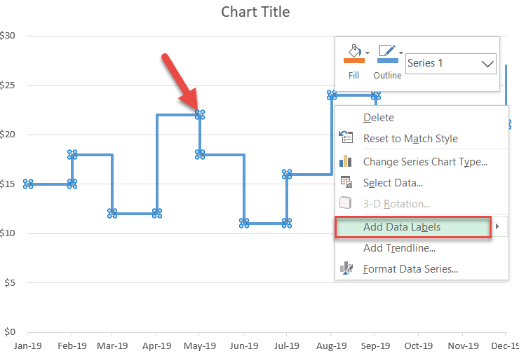
How to Create a Step Chart in Excel - Automate Excel
How to build a 100% stacked chart with percentages - Exceljet To add these to the chart, I need select the data labels for each series one at a time, then switch to "value from cells" under label options. Now we have a 100% stacked chart that shows the percentage breakdown in each column. Whenever you create these kind of helper calculations for a chart, take care with the Switch Column/Row button.

Enable or Disable Excel Data Labels at the click of a button - How To - PakAccountants.com
Format Data Labels in Excel- Instructions - TeachUcomp, Inc. Format Data Labels in Excel: Instructions. To format data labels in Excel, choose the set of data labels to format. One way to do this is to click the "Format" tab within the "Chart Tools" contextual tab in the Ribbon. Then select the data labels to format from the "Current Selection" button group.
Excel 3-D Pie charts - Microsoft Excel 2013
How to Add Percentages to Excel Bar Chart - Excel Tutorials To show our data like this, Charts are the most useful tool. We will present the charts and show you how can you add percentages to them in the example below. Contents 1 Create Chart from Data 2 Add Percentages to the Bar Chart 3 Clustered Column Create Chart from Data

Chapter 3 Excel 2007/2010 Charts
Solved: change data label to percentage - Power BI pick your column in the Right pane, go to Column tools Ribbon and press Percentage button do not hesitate to give a kudo to useful posts and mark solutions as solution LinkedIn Message 2 of 7 1,486 Views 1 Reply MARCreading Regular Visitor In response to az38 06-09-2020 09:03 AM Hi @az38, Thanks for your help!

Step by step to create a column chart with percentage change in Excel
How to use data labels - Exceljet When you check the box, you'll see data labels appear in the chart. If you have more than one data series, you can select a series first, then turn on data labels for that series only. You can even select a single bar, and show just one data label. In a bar or column chart, data labels will first appear outside the bar end.

How to Add Data Labels in Excel - Excelchat | Excelchat
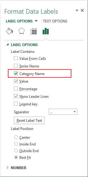
How to create a chart with both percentage and value in Excel? In the Format Data Labels pane, please check Category Name option, and uncheck Value option from the Label Options, and then, you will get all percentages and values are displayed in the chart, see screenshot: 15.
4.2 Formatting Charts – Beginning Excel
Count and Percentage in a Column Chart - ListenData Steps to show Values and Percentage 1. Select values placed in range B3:C6 and Insert a 2D Clustered Column Chart (Go to Insert Tab >> Column >> 2D Clustered Column Chart). See the image below Insert 2D Clustered Column Chart 2. In cell E3, type =C3*1.15 and paste the formula down till E6 Insert a formula 3.

Format Number Options for Chart Data Labels in PowerPoint 2011 for Mac
How do I show percentage data labels in Excel? - faq-ans.com Aug 15, 2021 — Then go to the stacked column, and select the label you want to show as percentage , then type = in the formula bar and select per...
How to Show Percentages in Stacked Bar and Column Charts in Excel
How to show percentages in stacked column chart in Excel? Add percentages in stacked column chart 1. Select data range you need and click Insert > Column > Stacked Column. See screenshot: 2. Click at the column and then click Design > Switch Row/Column. 3. In Excel 2007, click Layout > Data Labels > Center . In Excel 2013 or the new version, click Design > Add Chart Element > Data Labels > Center. 4.

410 How to display percentage labels in pie chart in Excel 2016 - YouTube
Excel, giving data labels to only the top/bottom X% values 1) Create a data set next to your original series column with only the values you want labels for (again, this can be formula driven to only select the top / bottom n values). See column D below. 2) Add this data series to the chart and show the data labels. 3) Set the line color to No Line, so that it does not appear! 4) Volia! See Below!
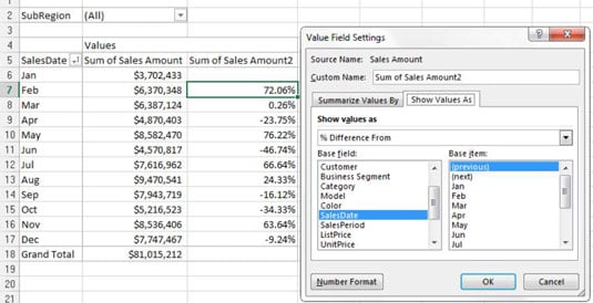
Create a Pivot Table Month-over-Month Variance View for Your Excel Report - dummies
How to visualize percentage progress in Excel Open the options for the Data Bar formatting you added and check Show Bar Only option. Click the OK buttons to apply the setting. Colored Icons Conditional Formatting has icons as well to visualize percentage progress. The first set of icons we want to show are color-based icons.
![Create Project Timeline Charts in Excel - [How To] + Free Template - PakAccountants.com](http://pakaccountants.com/wp-content/uploads/2014/08/timeline12.gif)
Create Project Timeline Charts in Excel - [How To] + Free Template - PakAccountants.com
Change the format of data labels in a chart - Microsoft Support To get there, after adding your data labels, select the data label to format, and then click Chart Elements > Data Labels > More Options. To go to the appropriate area, click one of the four icons ( Fill & Line, Effects, Size & Properties ( Layout & Properties in Outlook or Word), or Label Options) shown here.

How to Add Data Labels in Excel - Excelchat | Excelchat
how to calculate turnover percentage in excel - hojosoun.com Invoice template excel with vat. Gross Profit Percentage = ((Total Sale - Cost of Goods Sold) / Total sales) * 100 Gross Profit Percentage = (($3,000,000 - $650,000) / $3,000,000) * 100 Gross Profit Percentage = 78.33% In the Format Data Labels task pane, untick Value and tick the Percentage option to show only percentages.

Excel Graph Activities | Devpost

Solved: Power BI add manual input data in a table visual - Microsoft Power BI Community

microsoft excel - Chart fail to interpret dates for label values - Super User
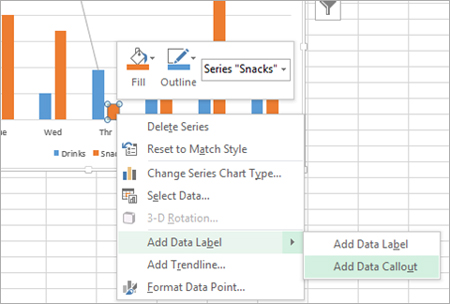
Adding rich data labels to charts in Excel 2013 - Microsoft 365 Blog

charts - Excel, giving data labels to only the top/bottom X% values - Stack Overflow
Post a Comment for "38 how to show data labels as percentage in excel"